PSense

Tutorial 2: Gradient Descent

Build Models in PSI

The following program implements the gradient descent algorithm:

def main(){
  x := [1.4,1.8,3.3,4.3,4.8,6.0,7.5,8.1,9.0,10.2];
  y := [2.2,4.0,6.1,8.6,10.2,12.4,15.1,15.8,18.4,20.0];
  w1 := 0;
  w2 := uniform(0, 1);
  a := 0.01;
  for t in [0..4){
    i := t;
    xi := x[i];
    yi := y[i];
    w1 = w1 - a*2*(w1+w2*xi-yi);
    w2 = w2 - a*2*(xi*(w1+w2*xi-yi));
  }
  return w2;
}

Here is what the program does:

• x and y are two arrays that store the observed data. The data come from the function $y = 2x$.

  x := [1,2,3,4,5,6,7,8,9,10];
  y := [2,4,6,8,10,12,14,16,18,20];
  

• We fit a simple linear regression model $y_i = w_1 + w_2x_i$. We first set the parameters $w_1$ and $w_2$ to some initial value. Then we use the gradient descent algorithm to adjust the parameters in order to minimize the error of current fit. To make the model simpler we set w1 a concrete initial value and assume w2 follows a uniform distribution:

  w1 := 0;
  w2 := uniform(0, 1);
  

• We set the learning rate a equal to 0.01. In each iteration we adjust the value of w1 and w2 so that the square error in the prediction moves against the gradient and towards the minimum. The algorithm is modified from this example in wikipedia. To make the model simpler, we only consider the prediction at a single value xi in each iteration.

  a := 0.01;
  for t in [0..8){
    i := t;
    xi := x[i];
    yi := y[i];
    w1 = w1 - a*2*(w1+w2*xi-yi);
    w2 = w2 - a*2*(xi*(w1+w2*xi-yi));
  }
  

• Finally we want to find out the distribution of the parameter w2 after 8 iterations.

  return w2;
  

• The results given by PSI in Wolfram Language is:

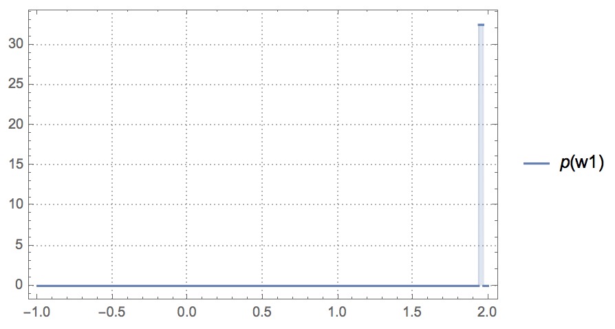
  p[w2_] := 59604644775390625000000/1832427479823270972979*Boole[-117376862070957979027021/59604644775390625000000+w2<=0]*Boole[-w2+57772217295567354027021/29802322387695312500000<=0]
  

  If we plot p[w2_] above, which is the probability density function of w2, we could see the value of w2 approaches to 2:

The code snippet can be found here.

Find Sensitivity with PSense

Notice that we initially suppose w2 follows a Uniform distribution with support $w2\in [0,1]$ (uniform(0,1)). We want to find out how the output distribution of w2 changes if we perturb the parameter of the prior distibution.

To estimate the change in the output distribution, we add disturbance ?eps to each parameter in uniform(0,1). Conceptually, we may have:

w2 := uniform(0+?eps, 1);     //Or, w2 := uniform(0, 1+?eps); 

Detailed definition of Sensitivity is in Tutorial 1.

PSense automatically adds ?eps to each constant parameters and find the sensitivity of the probabilistic program. Run the following in shell prompt:

psense -f examples/gradient_descent.psi

PSense would output the results for different metrics:

• Expectation Distance

Defined as $D_{Exp}=|\mathbb{E}[p_{eps}(r)]-\mathbb{E}[p(r)]|$, where $\mathbb{E}[p_{eps}(r)]$ and $\mathbb{E}[p(r)]$ are expectations of the output distributions with and without disturbance. After changing the first parameter, PSense genterates the symbolic expression for Expectation Distance as:

┌Analyzed parameter 1───────────────────┬
│         │ Expectation Distance        │
├─────────┼─────────────────────────────┼
│ Bounds  │ (80683972660613508548580146 │
│         │ 31573571*Abs[eps])/47683715 │
│         │ 820312500000000000000000000 │
│         │ 0                           │
│ Maximum │ 0.000169206554633 eps ->    │
│         │ 0.0100000000000 r1 ->       │
│         │ 1.90058660144               │
│ Linear  │ True                        │
└─────────┴─────────────────────────────┴

We can see the maximum value of the Expectation Distance is quite small. This is because after 8 iterations, the disturbance in the prior has little effect on the output distribution. We can try different iterations in PSense and plot the iterations against the maximum value of the Expectation Distance as:

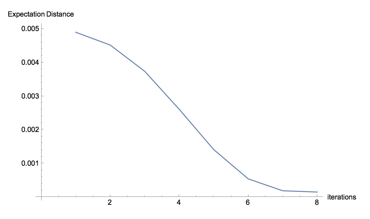
The more iterations the gredient descent algorithm takes, the less likely that eps in the prior parameter affects the output.

• Kolmogorov–Smirnov Statistic

Defined as $D_{KS}=\sup_{r\in support}|p_{eps}(r)-p(r)|$, where p_{eps}(r) and p(r) are cumulative density functions, and $\sup_{r\in support}$ represents the supremum of the distance over the support of $r$. PSense gives the distance $|p_{eps}(r)-p(r)|$ and the maximum value of $D_{KS}$, and then analyzes the linearity of $D_{KS}$.

┌Analyzed  parameter 1──────────────────┬
│         │ KS Distance                 │
├─────────┼─────────────────────────────┼
│ Bounds  │ Abs[44506960706629156649810 │
│         │ 0324588143317 - 23841857910 │
│         │ 1562500000000000000000000*r │
│         │ 1 - 45313800433235291735295 │
│         │ 8339219716888*Boole[2980232 │
│         │ 238769531250000000000000000 │
│         │ 0*r1 >= 5664225054154411466 │
│         │ 9119792402464611]*Boole[298 │
│         │ 023223876953125000000000000 │
│         │ 00000*r1 != 566422505415441 │
│         │ 14669119792402464611] + ((4 │
│         │ 450696070662915664981003245 │
│         │ 88143317 + 8068397266061350 │
│         │ 854858014631573571*eps - 23 │
│         │ 841857910156250000000000000 │
│         │ 0000000*r1 - 45313800433235 │
│         │ 2917352958339219716888*Bool │
│         │ e[2980232238769531250000000 │
│         │ 0000000000*r1 >= 5664225054 │
│         │ 1544114669119792402464611]* │
│         │ Boole[298023223876953125000 │
│         │ 00000000000000*r1 != 566422 │
│         │ 505415441146691197924024646 │
│         │ 11])*(Boole[445069607066291 │
│         │ 566498100324588143317 + 806 │
│         │ 839726606135085485801463157 │
│         │ 3571*eps <= 238418579101562 │
│         │ 500000000000000000000*r1] + │
│         │ Boole[298023223876953125000 │
│         │ 00000000000000*r1 >= 566422 │
│         │ 505415441146691197924024646 │
│         │ 11]*Boole[29802322387695312 │
│         │ 500000000000000000*r1 != 56 │
│         │ 642250541544114669119792402 │
│         │ 464611]))/(-1 + eps)]/80683 │
│         │ 972660613508548580146315735 │
│         │ 71                          │
│ Maximum │ 0.00990099009901 eps ->     │
│         │ -0.0100000000000 r1 ->      │
│         │ 1.86675723320               │
│ Linear  │ False                       │
└─────────┴─────────────────────────────┴

• Total Variation Distance

Defined as $D_{TVD}=\frac{1}{2}\int_{r\in support}\mid p_{eps}(r)-p(r)\mid$ for continuous distribution. PSense outputs the tightest linear upper and lower bound for the $D_{TVD}$ when the disturbance eps changes from 0 to 0.1:

┌Analyzed parameter 1─────────────────┐
│         │ TVD Bounds                │
├─────────┼───────────────────────────┤
│ Bounds  │ 2.2649885451518542*^-17 + │
│         │ 0.0013052896891758718*eps │
│         │ 0.00007758777570119023 +  │
│         │ 0.0013052896891758718*eps │
│ Maximum │ 0.0000846032773165 eps -> │
│         │ 0.0100000000000           │
│         │                           │
│ Linear  │ NA                        │
└─────────┴───────────────────────────┘

Yes, after 8 iterations, the TVD is close to 0. If we try only 4 iterations, we would get a larger TVD (run with -plain format).

TVD
TVD Bounds(lower, upper):
0.00012002414692527094 + 0.008312669864717516*eps
0.0003681905898401973 + 0.008312669864717516*eps
TVD Max
{0.0009585091693914027, {eps -> 0.09}}

Return to Tutorials